The BAK–TANG–WIESENFELD Sandpile
source page 85
General features
- First published by Bak, Tang, and Wiesenfeld (1987).
- Motivated by avalanching behaviour of a real sandpile.
- In one dimension rules represent downward movement of sand grains.
- Defined in any dimension, exactly solved (trivial) in one.
- Stochastic (bulk) drive, deterministic relaxation.
- Non-Abelian in its original definition.
- Many results actually refer to Dhar’s (1990a) Abelian sandpile, Sec. 4.2.
- Simple scaling behaviour disputed, multiscaling proposed.
- Exponents listed in Table 4.1, p. 92, are for the Abelian BTW Model.
Rules
- d dimensional (usually) hyper-cubic lattice and q the coordination number (on cubic lattices q = 2d).
- Choose (arbitrary) critical slope z^c = q − 1.
- Each site n ∈ {1,…, L}^d has slope z_n.
- Initialisation: irrelevant, model studied in the stationary state.
- Driving: add a grain at n0 chosen at random and update all uphill nearest neighbours n‘0 of n0: z_n0 →z_n0 + q/2 z_n0 →z_n‘0 − 1.
- Toppling: for each site n with z_n > z^c distribute q grains among its nearest neighbours n’ : z_n →z_n − q ∀n’.nn.n z_n →z_n + 1. In one dimension site n = L relaxes according to z_L → z_L − 1 z_L−1 → z_L−1 + 1.
- Dissipation: grains are lost at open boundaries.
- Parallel update: discrete microscopic time, sites exceeding zc at time t topple at t + 1 (updates in sweeps).
- Separation of time scales: drive only once all sites are stable, i.e. z_n ≤ z^c (quiescence).
- Key observables (see Sec. 1.3): avalanche sizes, the total number of topplings until quiescence; avalanche duration T , the total number of parallel updates until quiescence
[20]:
from SOC.models import BTW
Empty model
[21]:
b = BTW(L = 50, save_every = 50)
Running model
[22]:
b.run(200000, wait_for_n_iters = 100)
Waiting for wait_for_n_iters=100 iterations before collecting data. This should let the system thermalize.
[23]:
b.data_df.describe()
[23]:
| AvalancheSize | NumberOfReleases | number_of_iterations | |
|---|---|---|---|
| count | 200000.000000 | 200000.000000 | 200000.000000 |
| mean | 87.584035 | 92.235385 | 13.013605 |
| std | 251.254297 | 344.621080 | 32.636649 |
| min | 0.000000 | 0.000000 | 0.000000 |
| 25% | 0.000000 | 0.000000 | 0.000000 |
| 50% | 0.000000 | 0.000000 | 0.000000 |
| 75% | 27.000000 | 12.000000 | 7.000000 |
| max | 2337.000000 | 10060.000000 | 519.000000 |
[24]:
b.get_exponent(low = 2, high = 40)
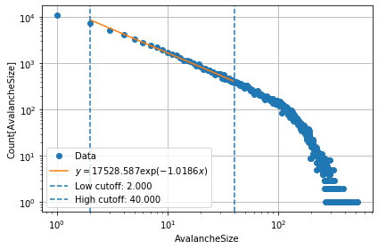
y = 17528.587 exp(-1.0186 x)
[24]:
{'exponent': -1.018594541688584, 'intercept': 4.243746902353518}
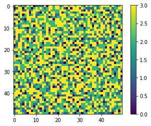
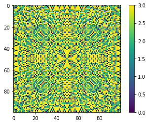
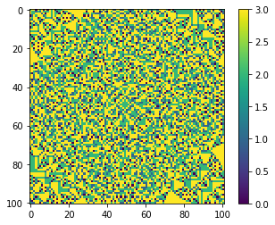
[25]:
b.plot_state();
[26]:
%matplotlib inline
a = BTW(30, save_every = 1)
a.run(10000)
Waiting for wait_for_n_iters=10 iterations before collecting data. This should let the system thermalize.
[27]:
a.animate_states(notebook = True)
Uniform model load
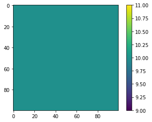
[28]:
c = BTW(100)
c.values[1:-1,1:-1] = 10
[29]:
c.plot_state();
[30]:
c.AvalancheLoop()
[30]:
{'AvalancheSize': 10000,
'NumberOfReleases': 28191892,
'number_of_iterations': 6920}
[31]:
c.plot_state();

Does pattern depend on height of load?
[32]:
for i in [4, 5, 6, 10, 20]:
mdl = BTW(100)
mdl.values[1:-1,1:-1] = i
mdl.AvalancheLoop()
mdl.plot_state();
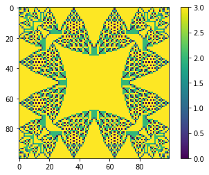
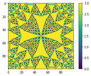
As we can see patter is changeing depending of pile height. Is there some maximum load?
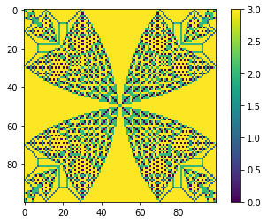
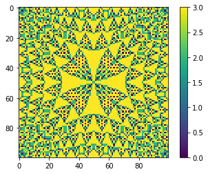
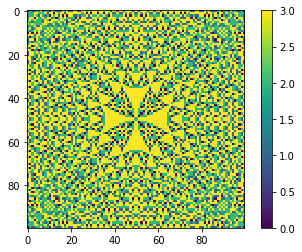
[33]:
mdl = BTW(100)
mdl.values[1:-1,1:-1] = 40
mdl.AvalancheLoop()
mdl.plot_state();

[34]:
mdl = BTW(100)
mdl.values[1:-1,1:-1] = 50
mdl.AvalancheLoop()
mdl.plot_state();
Pattern depends on load height.
Loading model in the single point at centr.
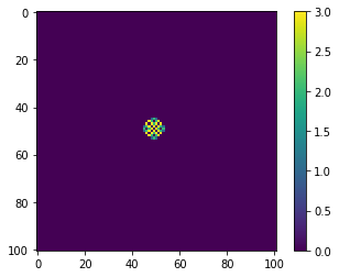
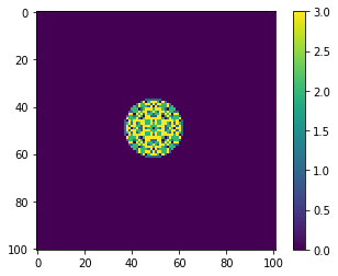
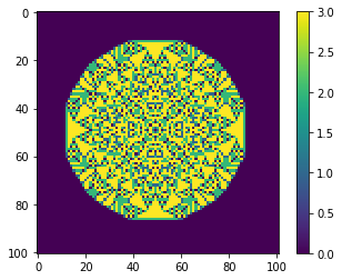
[35]:
for i in [10**2, 10**3, 10**4, 10**5]:
mdl = BTW(101)
mdl.values[50,50] = i
mdl.AvalancheLoop()
mdl.plot_state();
How exponent dependce on size of system?
[36]:
zip([10, 50, 100, 500],[1,1,1,1])
[36]:
<zip at 0x7fb61fdc2320>
[37]:
for l, w in zip([10, 50, 100, 200], [3*100**2, 3*100**2, 3*100**2, 5*100**2]):
mdl = BTW(L = l, save_every = 100)
mdl.run(2*w, wait_for_n_iters = w)
mdl.get_exponent(low = 2, high = 1.3*l)
Waiting for wait_for_n_iters=30000 iterations before collecting data. This should let the system thermalize.
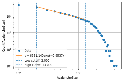
y = 6951.140 exp(-0.9537 x)
Waiting for wait_for_n_iters=30000 iterations before collecting data. This should let the system thermalize.
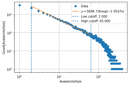
y = 5898.736 exp(-1.0567 x)
Waiting for wait_for_n_iters=30000 iterations before collecting data. This should let the system thermalize.
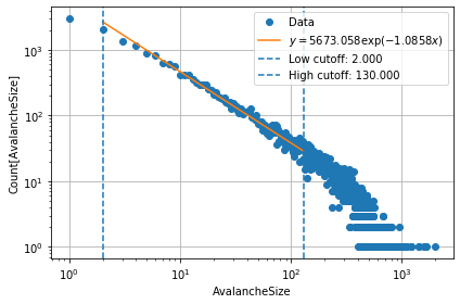
y = 5673.058 exp(-1.0858 x)
Waiting for wait_for_n_iters=50000 iterations before collecting data. This should let the system thermalize.
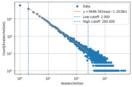
y = 9486.563 exp(-1.2028 x)